Method

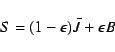
In the following discussion we use notation of Hauschildt (1992) and Paper I. The basic framework and the methods used for the formal solution and the solution of the scattering problem via operator splitting are discussed in detail in paper I and will thus not be repeated here. We have extended the framework to solve line transfer problems with a background continuum. The basic approach is similar to that of Hauschildt (1993). 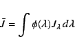In the simple case of a 2-level atom with background continuum we consider here as a test case, we use a wavelength grid that covers the profile of the line including the surrounding continuum. We then use the wavelength dependent mean intensities $J_\lambda$ and approximate $\Lambda$ operators $\ifmmode{\Lambda^*}\else\hbox{$\Lambda^*$}\fi$ to compute the profile integrated line mean intensities ${\bar J}$ and $\bar\ifmmode{\Lambda^*}\else\hbox{$\Lambda^*$}\fi$ via

$${\bar J}= \int \phi(\lambda) J_\lambda\,d\lambda$$

and

$$\bar\ifmmode{\Lambda^*}\else\hbox{$\Lambda^*$}\fi = \int \ph... ...bda) \ifmmode{\Lambda^*}\else\hbox{$\Lambda^*$}\fi \,d\lambda.$$

${\bar J}$ and $\bar\ifmmode{\Lambda^*}\else\hbox{$\Lambda^*$}\fi$ are then used to compute an updated value for ${\bar J}$ and the line source function

$$S = (1-\epsilon){\bar J}+\epsilon B$$

where $\epsilon$ is the line thermalization parameter ($0$ for a purely absorptive line, $1$ for a purely scattering line). $B$ is the Planck function, $B_\lambda$, profile averaged over the line

$$B = \int \phi(\lambda) B_\lambda\,d\lambda$$

via the standard iteration method

$$\left[1-\ifmmode{\Lambda^*}\else\hbox{$\Lambda^*$}\fi (1-\e... ...lse\hbox{$\Lambda^*$}\fi (1-\epsilon )\bar{\bar J_{\rm old}},$$

where ${\bar J_{\rm fs}}=\bar\Lambda {S_{\rm old}}$. This equation is solved directly to get the new values of ${\bar J}$ which is then used to compute the new source function for the next iteration cycle.

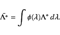
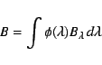
We construct the line $\bar\ifmmode{\Lambda^*}\else\hbox{$\Lambda^*$}\fi$ directly from the wavelength dependent $\ifmmode{\Lambda^*}\else\hbox{$\Lambda^*$}\fi$'s generated by the solution of the continuum transfer problems. For practical reasons, we use in this paper only the nearest neighbor $\ifmmode{\Lambda^*}\else\hbox{$\Lambda^*$}\fi$ discussed in paper I. Larger $\ifmmode{\Lambda^*}\else\hbox{$\Lambda^*$}\fi$s require significantly more storage and small test cases indicate that they do not decrease the number of iterations enough to warrant their use as long as they are not much larger than the nearest neighbor $\ifmmode{\Lambda^*}\else\hbox{$\Lambda^*$}\fi$.