Bibliography

Baron, E. & Hauschildt, P. H. 1998, ApJ, 495, 370

Cooperstein, J. & Baron, E. 1992, ApJ, 398, 531

Fabiani Bendicho, P., Trujillo Bueno, J., & Auer, L. 1997, A&A, 324, 161

Hauschildt, P. H. 1992, JQSRT, 47, 433

Hauschildt, P. H. 1993, JQSRT, 50, 301

Hauschildt, P. H. & Baron, E. 2006, A&A, 451, 273

Hubeny, I. & Burrows, A. 2006, ArXiv Astrophysics e-prints

Krumholz, M. R., Klein, R. I., & McKee, C. F. 2006, ArXiv Astrophysics e-prints

Lowrie, R. B. & Morel, J. E. 2001, JQSRT, 69, 475

Lowrie, R. B., Morel, J. E., & Hittinger, J. A. 1999, ApJ, 521, 432

Mihalas, D. & Klein, R. I. 1982, Journal of Computational Physics, 46, 97

Olson, G. L., Auer, L. H., & Buchler, J. R. 1987, JQSRT, 38, 431

Olson, G. L. & Kunasz, P. B. 1987, JQSRT, 38, 325

van Noort, M., Hubeny, I., & Lanz, T. 2002, ApJ, 568, 1066

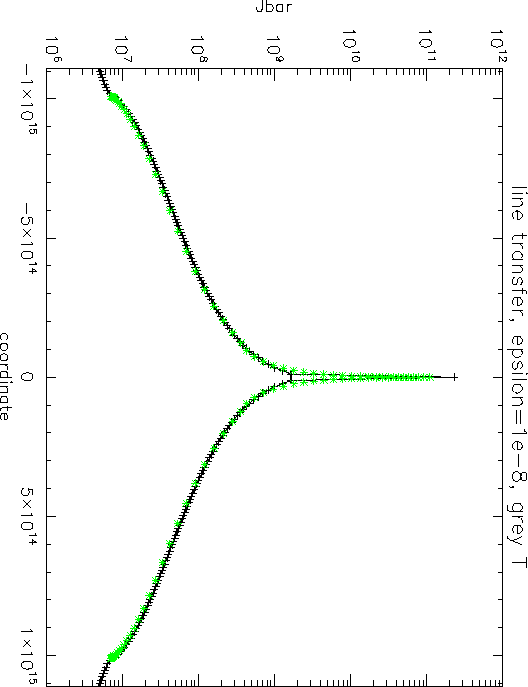
Figure 1: Comparison of the results obtained for the LTE line test with the 1D solver ($\times$ symbols) and the 3D line solver. This figure shows cuts along the $x$, $y$, and $z$ axes of the 3D grid for a grid with $n_x=n_y=n_z=2*64+1$ spatial points. The ordinate axis shows the coordinates, the $y$ axis the $\log$ of the mean intensity averaged over the line profiles (${\bar J}$) for cuts along the axes of the 3D grid. For the 1D comparison case the ordinate shows $\pm$ distance from the center.

Figure 2: Comparison of the results obtained for the LTE line test with the 1D solver ($+$ symbols) and the 3D line solver. The $x$ axis shows the distances from the center of the sphere, the $y$ axis the $\log$ of the mean intensity averaged over the line profiles (${\bar J}$). The 3D model uses $n_x=n_y=n_z=2*64+1$ spatial points.

Figure 3: Comparison of the results obtained for the $\epsilon _l=10^{-4}$ line test (constant $T$) with the 1D solver ($\times$ symbols) and the 3D line solver. This figure shows cuts along the $x$, $y$, and $z$ axes of the 3D grid with $n_x=n_y=n_z=2*64+1$ spatial points. The ordinate axis shows the coordinates, the $y$ axis the $\log$ of the mean intensity averaged over the line profiles (${\bar J}$) for cuts along the axes of the 3D grid. For the 1D comparison case the ordinate shows $\pm$ distance from the center.

Figure 4: Comparison of the results obtained for the $\epsilon _l=10^{-8}$ line test (constant $T$) with the 1D solver ($\times$ symbols) and the 3D line solver. This figure shows cuts along the $x$, $y$, and $z$ axes of the 3D grid with $n_x=n_y=n_z=2*64+1$ spatial points. The ordinate axis shows the coordinates, the $y$ axis the $\log$ of the mean intensity averaged over the line profiles (${\bar J}$) for cuts along the axes of the 3D grid. For the 1D comparison case the ordinate shows $\pm$ distance from the center.

Figure 5: Comparison of the results obtained for the $\epsilon _l=10^{-4}$ line test (grey $T$) with the 1D solver ($\times$ symbols) and the 3D line solver. This figure shows cuts along the $x$, $y$, and $z$ axes of the 3D grid with $n_x=n_y=n_z=2*96+1$ spatial points. The ordinate axis shows the coordinates, the $y$ axis the $\log$ of the mean intensity averaged over the line profiles (${\bar J}$) for cuts along the axes of the 3D grid. For the 1D comparison case the ordinate shows $\pm$ distance from the center.

Figure: Comparison of the results obtained for the $\epsilon _l=10^{-8}$ line test (grey $T$) with the 1D solver ($\times$ symbols) and the 3D line solver. This figure shows cuts along the $x$, $y$, and $z$ axes of the 3D grid with $n_x=n_y=n_z=2*64+1$ spatial points. The ordinate axis shows the coordinates, the $y$ axis the $\log$ of the mean intensity averaged over the line profiles (${\bar J}$) for cuts along the axes of the 3D grid. For the 1D comparison case the ordinate shows $\pm$ distance from the center.

Figure 7: Convergence of the iterations for the line transfer case with $\epsilon _l=10^{-2}$. The maximum relative corrections (taken over all spatial points) are plotted vs. iteration number.

Figure 8: Convergence of the iterations for the line transfer case with $\epsilon _l=10^{-4}$. The maximum relative corrections (taken over all spatial points) are plotted vs. iteration number.

Figure 9: Convergence of the iterations for the line transfer case with $\epsilon _l=10^{-8}$. The maximum relative corrections (taken over all spatial points) are plotted vs. iteration number.

Figure 10: Convergence of the iterations for the line transfer case with different $\epsilon _l$ as indicated in the legend. The maximum relative corrections (taken over all spatial points) are plotted vs. iteration number. The symbols without connecting lines are the convergence rates obtained without using Ng acceleration.