


Next: Formal solution
Up: Method
Previous: Radiative transfer equation
The mean intensity  is obtained from the source function
 by a formal solution of the RTE which is symbolically written
using the
by a formal solution of the RTE which is symbolically written
using the  -operator as
 |
(2) |
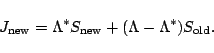
The source function is given by
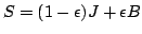 , where
  denotes the thermal coupling parameter and
  is Planck's function.
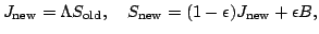
The -iteration method, i.e. to solve Eq. 2 by a fixed-point
iteration scheme of the form
 |
|
|
(3) |
fails in the case of large optical depths and small .
Here,  is the current estimate for the source
function and
is the current estimate for the source
function and  is new, improved, extimate of for the next
iteration. The failure to converge of the -iteration is caused
by the fact that the largest eigenvalue of the amplification matrix
is approximately (Mihalas et al., 1975)
is new, improved, extimate of for the next
iteration. The failure to converge of the -iteration is caused
by the fact that the largest eigenvalue of the amplification matrix
is approximately (Mihalas et al., 1975)
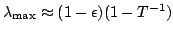 , where
  is the optical
thickness of the medium. For small and large , this is very close
to unity and, therefore, the convergence rate of the -iteration is very
poor. A physical description of this effect can be found in
Mihalas (1980).
is the optical
thickness of the medium. For small and large , this is very close
to unity and, therefore, the convergence rate of the -iteration is very
poor. A physical description of this effect can be found in
Mihalas (1980).
The idea of the ALI or operator splitting (OS) method is to reduce the
eigenvalues of the amplification matrix in the iteration scheme
(Cannon, 1973) by
introducing an approximate -operator (ALO)
 and to split according to
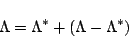 |
(4) |
and rewrite Eq. 3 as
 |
(5) |
This relation can be written as Hamann (1987)
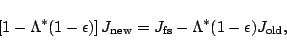 |
(6) |
where
 and
and
 is the current
estimate of the mean intensity . Equation 6 is solved to get the new values of
is the current
estimate of the mean intensity . Equation 6 is solved to get the new values of
 which is then used to compute the new
source function for the next iteration cycle.
which is then used to compute the new
source function for the next iteration cycle.
Mathematically, the OS method belongs to the same family of iterative
methods as the Jacobi or the Gauss-Seidel methods
(Golub & Van Loan, 1989). These
methods have the general form
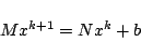 |
(7) |
for the iterative solution of a linear system  where the system
matrix
where the system
matrix  is split according to
  . In the case of the OS
method we have
. In the case of the OS
method we have
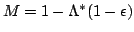 and, accordingly,
 for the system matrix
 . The
convergence of the iterations depends on the spectral radius,
. The
convergence of the iterations depends on the spectral radius,
 , of the iteration matrix
  . For convergence the
condition
. For convergence the
condition  must be fulfilled, this puts a restriction on
the choice of
. In general, the iterations will converge
faster for a smaller spectral radius. To achieve a significant
improvement compared to the -iteration, the operator
is
constructed so that the eigenvalues of the iteration matrix
must be fulfilled, this puts a restriction on
the choice of
. In general, the iterations will converge
faster for a smaller spectral radius. To achieve a significant
improvement compared to the -iteration, the operator
is
constructed so that the eigenvalues of the iteration matrix  are
much smaller than unity, resulting in swift convergence. Using
parts of the exact matrix (e.g., its diagonal or a tri-diagonal
form) will optimally reduce the eigenvalues of the
. The
calculation and the structure of
should be simple in order to
make the construction of the linear system in Eq. 6 fast. For
example, the choice
are
much smaller than unity, resulting in swift convergence. Using
parts of the exact matrix (e.g., its diagonal or a tri-diagonal
form) will optimally reduce the eigenvalues of the
. The
calculation and the structure of
should be simple in order to
make the construction of the linear system in Eq. 6 fast. For
example, the choice
 is best in view of the
convergence rate (it is equivalent to a direct solution by matrix inversion)
but the explicit construction of is more time
consuming than the construction of a simpler
. The solution of
the system Eq. 6 in terms of linear algebra, using modern
linear algebra packages such as, e.g., LAPACK (Anderson et al., 1992), is so fast that
its CPU time can be neglected for the small number of variables
encountered in 1D problems (typically the number of discrete shells
is about 50). However, for 2D or 3D problems the size of gets
very large due to the much larger number of grid points as compared to
the 1D case. Matrix inversions, which are necessary to solve
Eq. 6 directly, therefore become extremely time
consuming. This makes the direct solution of Eq. 6 more CPU intensive
even for
's of moderate bandwidth, except for the trivial case
of a diagonal
. Different methods like modified conjugate
gradient methods (Turek, 1993) may be effective for these
2D or 3D problems.
is best in view of the
convergence rate (it is equivalent to a direct solution by matrix inversion)
but the explicit construction of is more time
consuming than the construction of a simpler
. The solution of
the system Eq. 6 in terms of linear algebra, using modern
linear algebra packages such as, e.g., LAPACK (Anderson et al., 1992), is so fast that
its CPU time can be neglected for the small number of variables
encountered in 1D problems (typically the number of discrete shells
is about 50). However, for 2D or 3D problems the size of gets
very large due to the much larger number of grid points as compared to
the 1D case. Matrix inversions, which are necessary to solve
Eq. 6 directly, therefore become extremely time
consuming. This makes the direct solution of Eq. 6 more CPU intensive
even for
's of moderate bandwidth, except for the trivial case
of a diagonal
. Different methods like modified conjugate
gradient methods (Turek, 1993) may be effective for these
2D or 3D problems.
The CPU time required for the solution of the RTE using the OS method depends
on several factors: (a) the time required for a formal solution and the
computation of  , (b) the time needed to construct
, (c) the time
required for the solution of Eq. 6, and (d) the number of iterations
required for convergence to the prescribed accuracy. Points (a), (b) and (c)
depend mostly on the number of spatial points, and can be assumed to be fixed
for any given configuration. However, the number of iterations required to
convergence depends strongly on the bandwidth of
.
This indicates, that there is an optimum
bandwidth of the
-operator which will result in the shortest possible
CPU time needed for the solution of the RTE, see Hauschildt et al. (1994).
, (b) the time needed to construct
, (c) the time
required for the solution of Eq. 6, and (d) the number of iterations
required for convergence to the prescribed accuracy. Points (a), (b) and (c)
depend mostly on the number of spatial points, and can be assumed to be fixed
for any given configuration. However, the number of iterations required to
convergence depends strongly on the bandwidth of
.
This indicates, that there is an optimum
bandwidth of the
-operator which will result in the shortest possible
CPU time needed for the solution of the RTE, see Hauschildt et al. (1994).
Next: Formal solution
Up: Method
Previous: Radiative transfer equation
Peter Hauschildt
2006-01-09