Formal solution

The formal solution through the voxel grid can be performed by a variety of methods. So far, we have implemented both a short-characteristic (SC, Olson et al., 1987) and a long-characteristic (LC) method. Long and short characteristics are shown schematically in Fig. 1. In our current implementation, the long characteristics are followed continuously through the voxel grid, the short characteristics start at the center of a voxel and step closest to the center of the next voxel. The distances along a (short or long) characteristic are then used to compute the optical depth steps. Along a characteristic (either short or long), the formal solution is computed using a piece-wise parabolic (PPM) or piece-wise linear (PLM) interpolation and integration of the source function (Olson & Kunasz, 1987). Auer (2003) discusses the effect that high order interpolation may cause problems, therefore, we automatically use piece-wise linear interpolation if the change in the source function along the 3 points of the PPM step would be larger than a prescribed threshold (typically factors of 100) or if the optical depth along the characteristic is very small (typically less than $10^{-3}$). Depending on the direction $(\theta,\phi)$ of the characteristic, the formal solution proceeds through the voxel grid.

Therefore, along a characteristic [which is in the static case just a straight line with given $(\theta,\phi)$] the transport equation is simply

$${d I\over d\tau} = I - S$$ (8)

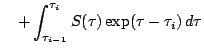
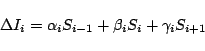
With this definition, the formal solution of the RTE along the characteristics can be written in the following way (cf. Olson & Kunasz, 1987, for a derivation of the formulae) where we have suppressed the index labeling the characteristic; $\tau_i$ denotes the optical depth along the characteristic with $\tau_1\equiv 0$ and $\tau_{i-1} \le \tau_i$ while $\tau$ is calculated using piecewise linear interpolation of $\chi$ along the characteristic, viz.

$$I(\tau_i) = I(\tau_{i-1}) \exp(\tau_{i-1}-\tau_i)$$

$$\quad +\int_{\tau_{i-1}}^{\tau_i} S(\tau) \exp(\tau-\tau_i) \, d\tau$$ (9)

$$I(\tau_i) \equiv I_{i-1}\exp(-\Delta\tau_{i-1})+\Delta I_i$$ (10)

$i$ labels the points along a characteristic and $\Delta\tau_{i}$ is calculated using piecewise linear interpolation of $\chi$ along the characteristic

$$\Delta\tau_{i-1} = (\chi_{i-1}+\chi_i)\vert s_{i-1}-s_i\vert/2$$ (11)

The starting points of each characteristic are at the center of the voxels on their starting faces of the voxel grid.

The source function $S(\tau)$ along a characteristic is interpolated by linear or parabolic polynomials so that

$$\Delta I_i = \alpha_i S_{i-1} + \beta_i S_i + \gamma_i S_{i+1}$$ (12)

with

$$\alpha_i = e_{0i} + [e_{2i}-(\Delta\tau_i+2\Delta\tau_{i-1})e_{1i}]$$

$$\qquad /[\Delta\tau_{i-1}(\Delta\tau_i+\Delta\tau_{i-1})]$$ (13)

$$\beta_i = [(\Delta\tau_i+\Delta\tau_{i-1})e_{1i}-e_{2i}] /[\Delta\tau_{i-1}\Delta\tau_i]$$ (14)

$$\gamma_i = [e_{2i}-\Delta\tau_{i-1}e_{1i}] /[\Delta\tau_i(\Delta\tau_i+\Delta\tau_{i-1})]$$ (15)

for parabolic interpolation and

$$\alpha_i = e_{0i} - e_{1i}/\Delta\tau_{i-1}$$ (16)

$$\beta_i = e_{1i}/\Delta\tau_{i-1}$$ (17)

$$\gamma_i = 0$$ (18)

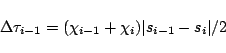
for linear interpolation. The auxiliary functions are given by

$$e_{0i} = 1-\exp(-\Delta\tau_{i-1})$$ (19)

$$e_{1i} = \Delta\tau_{i-1} - e_{0i}$$ (20)

$$e_{2i} = (\Delta\tau_{i-1})^2 - 2e_{1i}$$ (21)

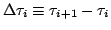and $\Delta\tau_i \equiv \tau_{i+1}-\tau_i$ is the optical depth along the characteristic from point $i$ to point $i+1$. The linear coefficients have to be used (at least) at the last integration point along each characteristic, and for some cases it might be better to also use linear interpolation for some inner points so as to ensure stability.

The integration over solid angle can be done in the static case using a simple Simpson or trapezoidal quadrature formula. However, in the case of Lagrangian frame radiation transport, the angles $(\theta,\phi)$ vary along a (curved) characteristic. Therefore, the $(\theta,\phi)$ grid changes for each voxel and developing a quadrature formula in advance requires a pass through all voxels, storing all $(\theta,\phi)$ points for each of them. For larger grids this will amount to substantial long term memory requirements as the resulting quadrature weights will have to be stored for each $(\theta,\phi)$ pair at all voxels. To avoid this, we have implemented a simple Monte-Carlo (MC) scheme to perform the integration over solid angle. 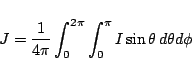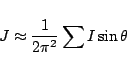In the MC integration, the integral

$$J = \frac{1}{4\pi} \int_0^{2\pi} \int_0^{\pi} I \sin\theta\,d\theta d\phi$$

is replaced by a simple MC sum of the form

$$J \approx \frac{1}{2\pi^2} \sum I \sin\theta$$

where the sum goes over all solid angle points $(\theta,\phi)$. The $(\theta,\phi)$ are randomly selected and given equal weight in the MC sums. This also works for precribed $(\theta,\phi)$ grids as long as the number of $(\theta,\phi)$ points is sufficiently large. The accuracy is improved by maintaining the normalization numerically for a unity valued test function. The MC method has the advantage that the solid angle points can vary from voxel to voxel (important for configurations with velocity fields where the transfer equation is solved in the locally co-moving frame). In the static case, the accuracy of the MC method is only insignificantly worse than that of the deterministic quadrature, which indicates that the MC integration will be very useful in the case of 3D radiation transport in moving media.