Bibliography

Adam, J. 1990, A&A, 240, 541

Anderson, E., Bai, Z., Bischof, C., et al. 1992, LAPACK Users' Guide (SIAM)

Auer, L. 2003, in Stellar Atmosphere Modeling, ed. I. Hubeny, D. Mihalas, & K. Werner, Vol. 288 (San Franscisco: ASP Conf. Series), 3

Auer, L., Fabiani Bendicho, P., & Trujillo Bueno, J. 1994, A&A, 292, 599

Cannon, C. J. 1973, JQSRT, 13, 627

Dykema, P. G., Klein, R. I., & Castor, J. I. 1996, ApJ, 457, 892

Fabiani Bendicho, P., Trujillo Bueno, J., & Auer, L. 1997, A&A, 324, 161

Golub, G. H. & Van Loan, C. F. 1989, Matrix computations (Baltimore: Johns Hopkins University Press)

Hamann, W.-R. 1987, in Numerical Radiative Transfer, ed. W. Kalkofen (Cambridge University Press), 35

Hauschildt, P. H. 1992, JQSRT, 47, 433

Hauschildt, P. H. & Baron, E. 2004, , 417, 317

Hauschildt, P. H., Störzer, H., & Baron, E. 1994, JQSRT, 51, 875

Hummel, W. 1994a, Astrophys. Space. Sci., 216, 87

Hummel, W. 1994b, A&A, 289, 458

Hummel, W. & Dachs, J. 1992, A&A, 262, L17

Mihalas, D. 1978, Stellar Atmospheres (New York: W. H. Freeman)

Mihalas, D. 1980, ApJ, 237, 574

Mihalas, D., Kunasz, P., & Hummer, D. 1975, ApJ, 202, 465

Ng, K. C. 1974, J. Chem. Phys., 61, 2680

Norman, M. L. 2000, in Revista Mexicana de Astronomia y Astrofisica Conference Series, Vol. 9, 66-71

Olson, G. L., Auer, L. H., & Buchler, J. R. 1987, JQSRT, 38, 431

Olson, G. L. & Kunasz, P. B. 1987, JQSRT, 38, 325

Papkalla, R. 1995, A&A, 295, 551

Rijkhorst, E.-J., Plewa, T., Dubey, A., & Mellema, G. 2005, A&A, in press, astro-ph/0505213

Steiner, O. 1991, A&A, 242, 290

Trujillo Bueno, J. & Fabiani Bendicho, P. 1995, ApJ, 455, 646

Turek, S. 1993, preprint

van Noort, M., Hubeny, I., & Lanz, T. 2002, ApJ, 568, 1066

Vath, H. M. 1994, A&A, 284, 319

Xiaoye, S. L. & Demmel, J. W. 2003, ACM Transaction on Mathematical Software, 29, 110

Zurmühl, R. & Falk, S. 1986, Matrizen und ihre Anwendungen, 5th edn., Vol. 2 (Berlin: Springer-Verlag)

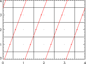
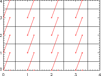
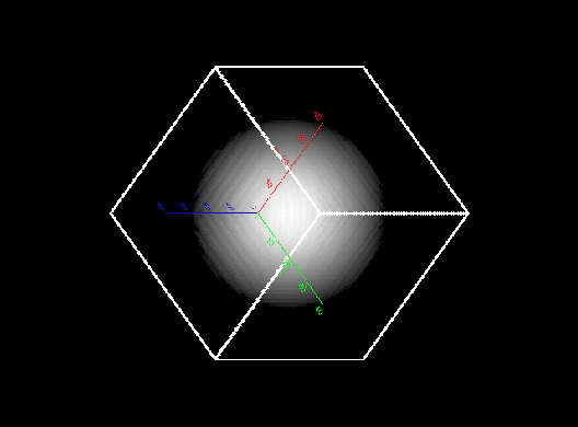
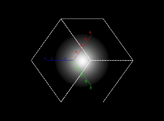
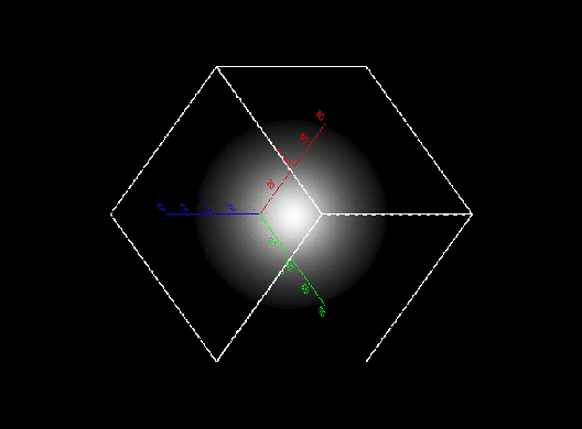
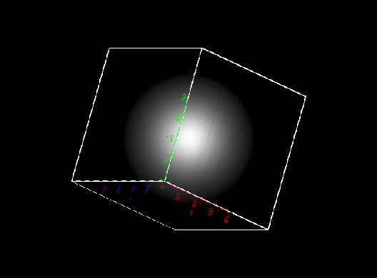
Figure 1: Schematic sketch of the different types of characteristics used in the framework. The left panel shows the long characteristics, the right panel the short characteristics. The voxel boundaries and centers ('$+$' symbols) are indicated. The '$+$' denote the points between which the geometric distance is used to compute optical depth steps.

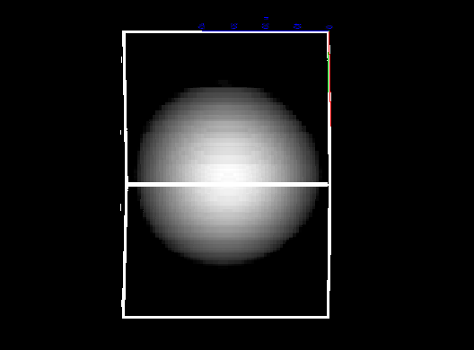
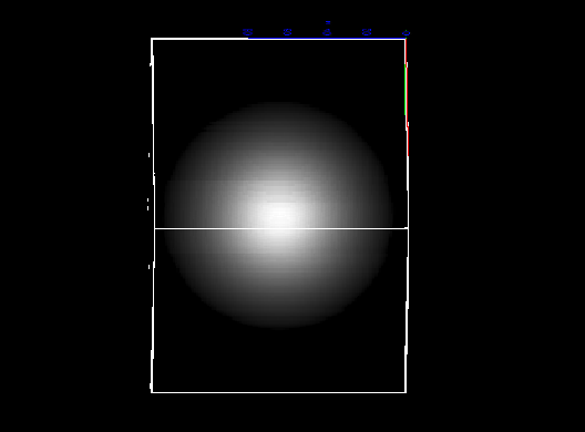
Figure 2: Comparison of the results obtained for the LTE test with the 1D solver ($+$ symbols) and the 3D solver. The $x$ axis shows the distances from the center of the sphere, the $y$ axis the $\log$ of the mean intensity.

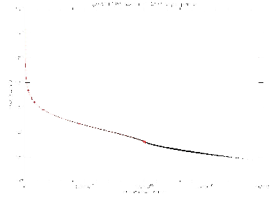Figure 3: Comparison of the results obtained for the scattering dominated ( $\epsilon =10^{-4}$) test with the 1D solver ($+$ symbols) and the 3D solver. The $x$ axis shows the distances from the center of the sphere, the $y$ axis the $\log$ of the mean intensity. The top panel shows the results for a (spatial; solid angle) grid with $(193^3; 64^2)$ points, the middle panel for $(129^3; 64^2)$ points and the bottom panel for $(129^3; 16^2)$ points.

Figure 4: Mean intensity contour plots for the test case with $\epsilon =10^{-4}$ with $129^3$ spatial points and $16^2$ (left panel) and $64^2$ solid angle points. The axes are labeled by voxel index with $(x,y,z) = (0,0,0)$ being the center of the voxel grid. Each plot shows one outside face of the voxel cube (the physical scales are the same in all directions).

Figure 5: Mean intensity surfaces at the $z-y$ face for the test case with $\epsilon =10^{-4}$, $129^3$ spatial points, and $16^2$ (left panel) and $64^2$ solid angle points. The axes are labeled by voxel index with $(x,y,z) = (0,0,0)$ being the center of the voxel grid. Each plot shows one outside face of the voxel cube (the physical scales are the same in all directions).

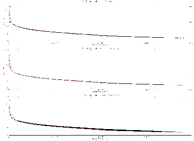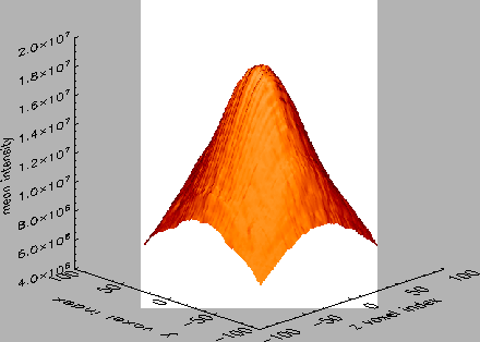
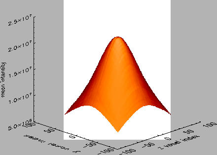
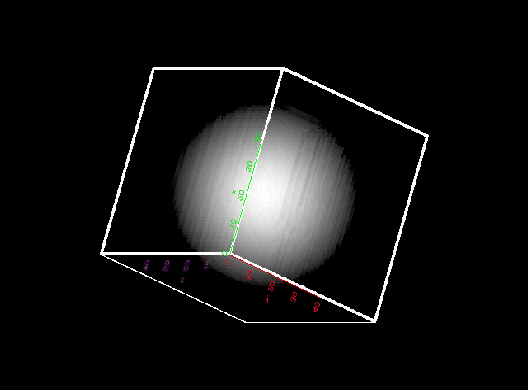
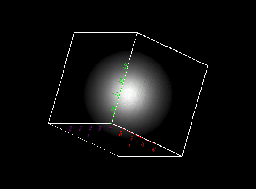
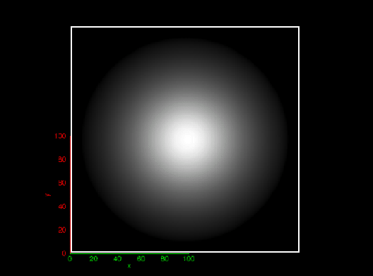
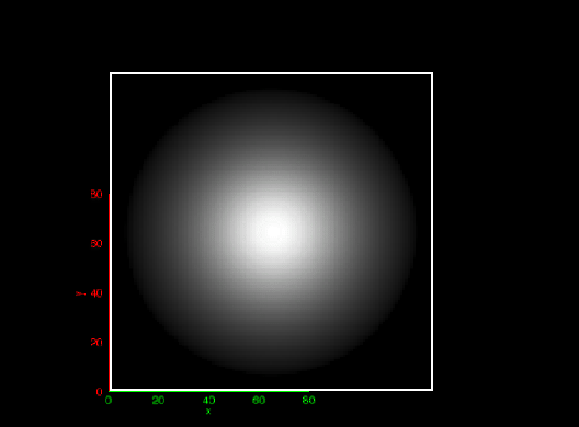
Figure 6: Mean intensity surface at the $z-y$ face for the test case with $\epsilon =10^{-4}$ with $193^3$ spatial points and $64^2$ solid angle points. The axes are labeled by voxel index with $(x,y,z) = (0,0,0)$ being the center of the voxel grid.

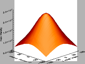Figure 7: Convergence properties of the codes for the $\epsilon =10^{-4}$ test case. The labels indicate the different methods used. The 3D test runs use $65^3$ spatial and $16^2$ angular points.

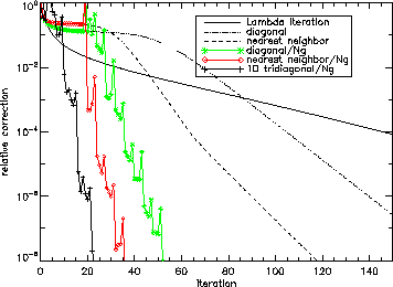Figure 8: Convergence properties of the codes for the $\epsilon =10^{-4}$ test case and different grid sizes. The labels indicate the different grid sizes used, all but the $\Lambda$ iteration use the nearest neighbor operator with Ng acceleration.

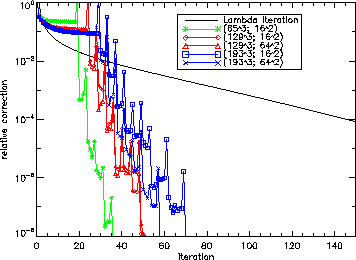Figure 9: Convergence properties of the $\epsilon =10^{-4}$ test case for various $\ifmmode{\Lambda^*}\else\hbox{$\Lambda^*$}\fi$ operator bandwidth choices with and without Ng acceleration.

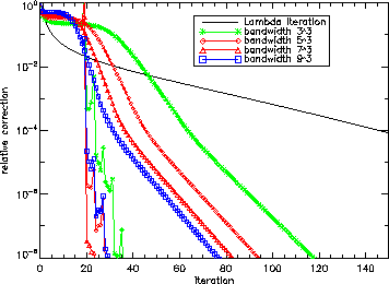Figure 10: Comparison of the results obtained for the scattering dominated ( $\epsilon =10^{-8}$) test with the 1D solver ($+$ symbols) and the 3D solver. The $x$ axis shows the distances from the center of the sphere, the $y$ axis the $\log$ of the mean intensity. The graph shows the results for a (spatial; solid angle) grid with $(129^3; 64^2)$ points. Note the large dynamic range (12 dex) of the mean intensities.

Figure 11: Comparison of the results obtained for the scattering dominated ( $\epsilon =10^{-8}$) test with the 1D solver ($+$ symbols) and the 3D solver for slices along the $x$, $y$, and $z$ axes. The plot shows the results for a (spatial; solid angle) grid with $(129^3; 64^2)$ points. Note the large dynamic range (12 dex) of the mean intensities.

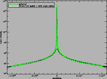Figure 12: Convergence properties of the codes for the $\epsilon =10^{-8}$ test case. The labels indicate the different methods used. These test runs use $65^3$ spatial and $16^2$ angular points.

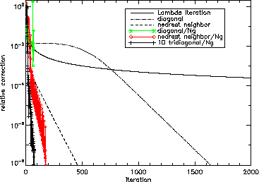Figure 13: Convergence properties of the codes for the $\epsilon =10^{-8}$ test case and different angular grid sizes. The labels indicate the different grid sizes used, all but the $\Lambda$ iteration use the nearest neighbor operator with Ng acceleration.

Figure 14: Visualization of the results for the LTE case. The voxel grid has $65^3$ elements. The intensity image is shown for $(\theta ,\phi ) = (0,0)$ (upper left panel), $(45,45)$ (bottom right panel), $(140,250)$ (upper right panel), and $(89,139)$ (bottom right panel) degrees. The intensities are mapped linearly to 255 shades of gray. The direction of the axes are given with axes lengths corresponding to a total of 50 voxels. The borders of the front faces of the voxel cube are shown, their widths corresponds to the apparent width of a voxel. Note that the different panels are at different scales.

Figure 15: Visualization of the results for the $\epsilon =10^{-4}$ case with a $129^3$ elements voxel grid. The intensity image is shown for $(\theta ,\phi ) = (0,0)$ (upper left panel), $(45,45)$ (bottom right panel), $(140,250)$ (upper right panel), and $(89,139)$ (bottom right panel) degrees. The intensities are mapped linearly to 255 shades of gray. The direction of the axes are given with axes lengths corresponding to a total of 100 voxels. The borders of the front faces of the voxel cube are shown, their widths corresponds to the apparent width of a voxel. Note that the different panels are at different scales.

Figure 16: Visualization of the results for the $\epsilon =10^{-4}$ case with a $193^3$ voxel grid. The intensity image is shown for $(\theta ,\phi ) = (0,0)$ (upper left panel), $(45,45)$ (bottom right panel), $(140,250)$ (upper right panel), and $(89,139)$ (bottom right panel) degrees. The intensities are mapped linearly to 255 shades of gray. The direction of the axes are given with axes lengths corresponding to a total of 100 voxels. The borders of the front faces of the voxel cube are shown, their widths corresponds to the apparent width of a voxel. Note that the different panels are at different scales.

Figure 17: Visualization of the results for the $\epsilon =10^{-8}$ case with a $129^3$ elements voxel grid. The intensity image is shown for $(\theta ,\phi ) = (0,0)$ (upper left panel), $(45,45)$ (bottom right panel), $(140,250)$ (upper right panel), and $(89,139)$ (bottom right panel) degrees. The intensities are mapped linearly to 255 shades of gray. The direction of the axes are given with axes lengths corresponding to a total of 100 voxels. The borders of the front faces of the voxel cube are shown, their widths corresponds to the apparent width of a voxel. Note that the different panels are at different scales.

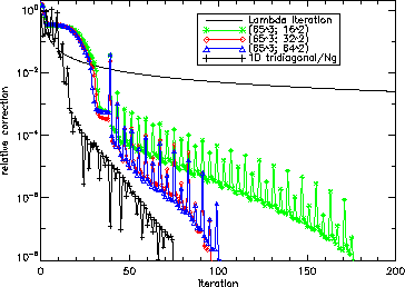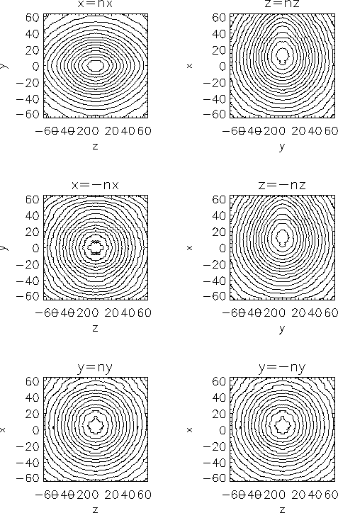
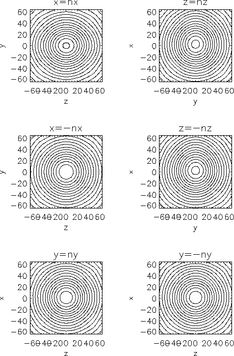
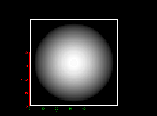
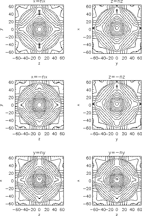
Figure 18: Scaling properties of the MPI version of the 3D RT code for parallel clusters based on Opterons and G5 CPUs. In absolute scales the G5s are about 30% faster than the Opterons.

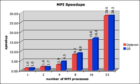Figure 19: Comparison of the mean intensity contour plots for the test case with $\epsilon =10^{-4}$ with $129^3$ spatial points and $64^2$ solid angle points. The left panel shows the results obtained with the short characteristics method whereas the right panel shows the results of the long characteristics method. The axes are labeled by voxel index with $(x,y,z) = (0,0,0)$ being the center of the voxel grid. Each plot shows one outside face of the voxel cube (the physical scales are the same an all directions).

Figure 20: Comparison of the mean intensity surfaces at the $z-y$ face for the test case with $\epsilon =10^{-4}$ with $129^3$ spatial points and $64^2$ solid angle points. The left panel shows the results obtained with the short characteristics methods whereas the right panel shows the results of the long characteristics method. The axes are labeled by voxel index with $(x,y,z) = (0,0,0)$ being the center of the voxel grid. Each plot shows one outside face of the voxel cube (the physical scales are the same in all directions).