

Next: About this document ...
Up: Spherically symmetric model atmospheres
Previous: References
Figure:
Comparison of
the models presented in this paper (full line) to NG-giant models
(dotted line) in the optical spectrum. The resolution has been
reduced to  . The top panel shows models with
 , the bottom panel for
  , both sets have
 and solar abundances.
 |
Figure:
Comparison of
the models presented in this paper (full line) to NG-giant models
(dotted line) in the near IR spectral range. The resolution has been
reduced to  . The top panel shows models with
 , the middle panel shows
  , and
the bottom panel for
  , all three sets have
 and solar abundances.
 |
Figure 3:
Models with multiple radiative/convective zones.
Each point marks a model that has multiple radiative/convective zones.
To minimize the number of figures we plotted all metallicities
in one graph and used different symbols for different metallicities
as indicated in the figure.
The log(g) values for sub- and super-solar metallicities have
been slightly shifted to keep the figure legible.
Note the continuous distribution of models with
multiple radiative/convective zones, which is also
continuous is metallicity space.
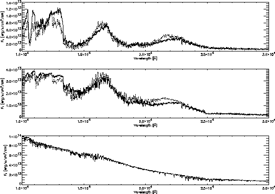 |
Figure:
Absorption coefficients versus optical depth at 1.2.
All models have z=-0.3 and log(g)=2.5. The effective temperature
of the models are from top to bottom 2800 K, 3000 K, 3200 K and
3400 K.
The cross hatched regions are the convective zones.
For reference, we indicate the gas pressure and the gas temperature
at the respective optical depth at the top of each figure.
To the right we labeled the most important opacity sources.
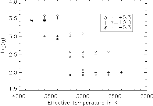 |
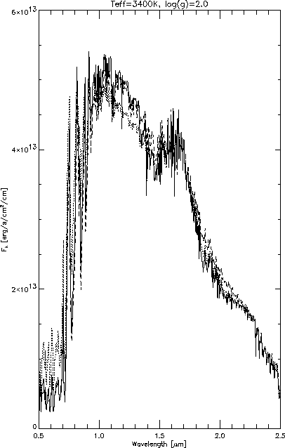
Figure:
Comparison of
low-resolution (about  ) synthetic spectra for models with
  ,
,
 and solar abundances (full line),
 ![$[{\rm M/H}]=-0.3$](img12.gif) (dotted line)
and
(dotted line)
and ![$[{\rm M/H}]=+0.3$](img11.gif) (dashed line).
(dashed line).
 |
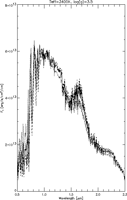
Figure:
Comparison of
low-resolution (about  ) synthetic spectra for models with
  ,
,
 and solar abundances (full line),
 ![$[{\rm M/H}]=-0.3$](img12.gif) (dotted line)
and
(dotted line)
and ![$[{\rm M/H}]=+0.3$](img11.gif) (dashed line).
(dashed line).
 |
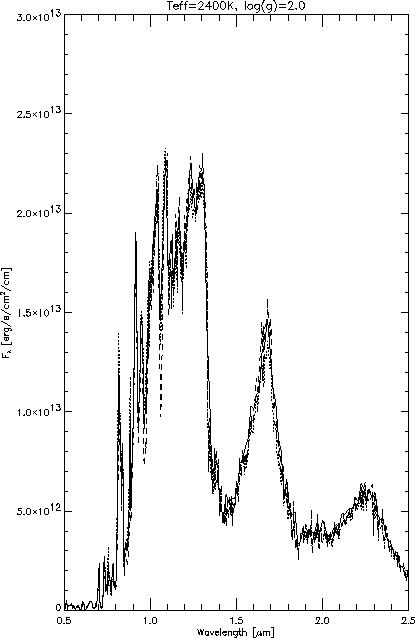
Figure:
Comparison of
low-resolution (about  ) synthetic spectra for models with
  ,
,
 and solar abundances (full line),
 ![$[{\rm M/H}]=-0.3$](img12.gif) (dotted line)
and
(dotted line)
and ![$[{\rm M/H}]=+0.3$](img11.gif) (dashed line).
(dashed line).
 |
Figure:
Comparison of
low-resolution (about  ) synthetic spectra for models with
  ,
,
 and solar abundances (full line),
 ![$[{\rm M/H}]=-0.3$](img12.gif) (dotted line)
and
(dotted line)
and ![$[{\rm M/H}]=+0.3$](img11.gif) (dashed line).
(dashed line).
 |


Next: About this document ...
Up: Spherically symmetric model atmospheres
Previous: References
Peter H. Hauschildt
8/30/2000
