


Next: About this document ...
Up: The NextGen Model Atmosphere
Previous: References
Figure:
Temperature structures for solar abundance models with
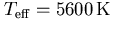 ,
,  , and
, and  for varying gravities (as indicated).
 is the optical
depth in the continuum (b-f and f-f processes) at a wavelength of
is the optical
depth in the continuum (b-f and f-f processes) at a wavelength of  m.
m.
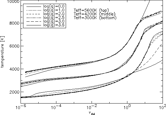 |
Figure:
Radial extensions  for solar abundance models with
, , and (as indicated).
for solar abundance models with
, , and (as indicated).
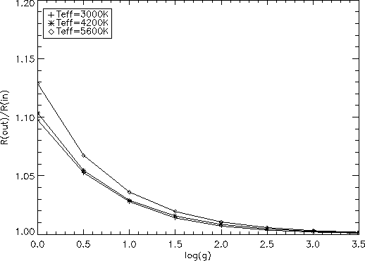 |
Figure:
Comparison between solar abundance giant models
calculated using spherical geometry and radiative transfer (full curves) and
plane parallel geometry and radiative transfer(dotted curves) in the
blue/optical spectral region. The resolution of the spectra has been reduced to
 .
.
 |
Figure:
Relative flux change between spherical and plane parallel
model calculations. The y-axis shows (fp-fs)/fs, where fp is the flux of
the plane parallel model and fs is the flux calculated for the spherical model.
The resolution of the spectra was reduced to .
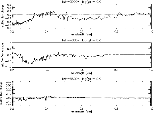 |
Figure:
Relative flux change between spherical and plane parallel
model calculations. The y-axis shows (fp-fs)/fs, where fp is the flux of
the plane parallel model and fs is the flux calculated for the spherical model.
The resolution of the spectra is  .
.
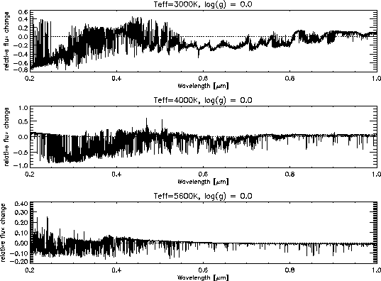 |
Figure:
Relative flux change between spherical and plane parallel
model calculations. The y-axis shows (fp-fs)/fs, where fp is the flux of
the plane parallel model and fs is the flux calculated for the spherical model.
The resolution of the spectra was reduced to .
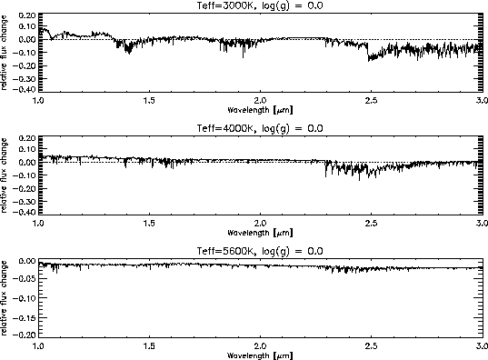 |
Figure:
Relative flux change between spherical and plane parallel
model calculations. The y-axis shows (fp-fs)/fs, where fp is the flux of
the plane parallel model and fs is the flux calculated for the spherical model.
The resolution of the spectra is .
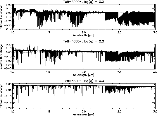 |
Figure:
Temperature structures for spherical (full curves)
and plane parallel (dotted lines) model calculations. is the optical
depth in the continuum (b-f and f-f processes) at a wavelength of m.
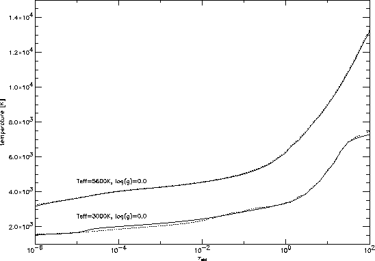 |
Figure:
Sensitivity of the synthetic spectra to gravity
changes for solar abundance models with , , and (as indicated). The resolution of the spectra has been reduced to .
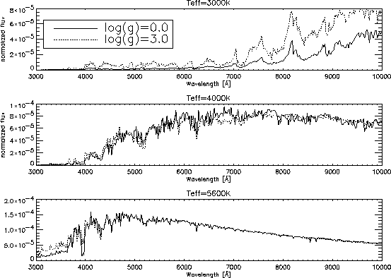 |
Figure:
Sensitivity of the synthetic spectra to metallicity
changes for models with , , and  (as indicated) and
  . For the
  model the metallicities
![$[{\rm M/H}]=0.0$](img61.gif) and
and ![$[{\rm M/H}]=-0.3$](img23.gif) are shown whereas for the hotter two models the
metallicities shown are and
are shown whereas for the hotter two models the
metallicities shown are and ![$[{\rm M/H}]=-0.7$](img62.gif) .The resolution of the spectra has been reduced to .
.The resolution of the spectra has been reduced to .
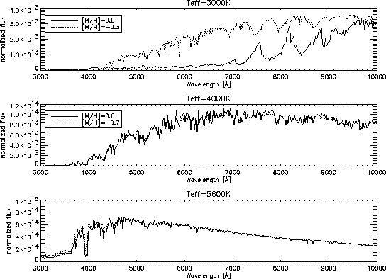 |
Figure:
Synthetic spectra at resolution
for models with  , , solar abundances, and
stellar masses of
, , solar abundances, and
stellar masses of  and
and  .
.
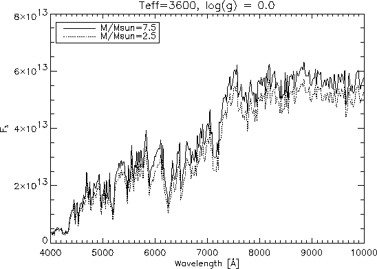 |
Figure:
Overview over selected departure coefficients
for a NLTE model with  , , and solar abundances.
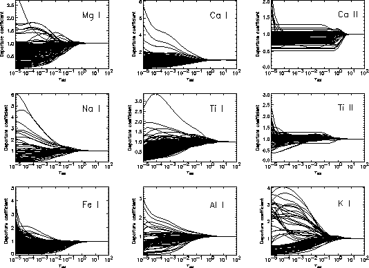 |
Figure:
Overview over selected departure coefficients
for a NLTE model with , , and solar abundances.
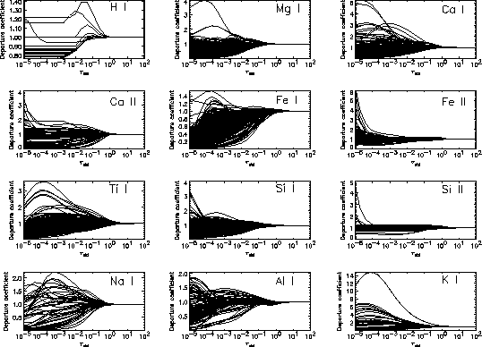 |
Next: About this document ...
Up: The NextGen Model Atmosphere
Previous: References
Peter H. Hauschildt
7/14/1999